OVERVIEW
System compensation refers to the digital correction methodology utilized to compensate for typical output system characteristics. Compensation is needed to ensure that the generated output signal properly represents the desired reference specification. The reference specification can be based on either time domain (e.g. Shock/SRS synthesis or Field Data Replication) or frequency domain definitions (e.g. Sine on Random or Random on Random).

This discussion serves as a basic overview to help understand the process and to aid in operation of the software and the several user controllable parameters. As noted earlier, the compensation process is invoked from several Spectral Dynamics control applications including Shock, Field Data Replication, Sine on Random and Random on Random.

BACKGROUND
The fundamental process is based on a model of the system frequency response (transfer) function. In this model, the excitation of an object is modified by that object’s transfer function which then changes that excitation into an observable response. By simple linear extension, if we can measure the response as well as the input excitation, one can estimate what the system characteristics are. Once the model is calculated, one can then take a defined reference and reproduce that reference as a system output by compensating the reference for the system’s frequency response function.

The process of determining the system’s transfer function model is called System ID. The process generally utilizes a measured controlled excitation and the associated excitation output response. The purpose is to define the frequency response function of the output sub system (typically a shaker/amplifier unit). The calculations are performed in the frequency domain which means that the bandwidth of the measurements is generally matched to the bandwidth of the desired reference signal. The reference signal is typically a time domain waveform of user generated properties and content.

Based on the above description, several critical assumptions are made in the processing/development of the compensation function. The first is that the system must respond in a linear manner and be time invariant. In this context one must expect that the output system characteristics are stable. Some variations with time can be incorporated into the compensation function, but in general, must be somewhat limited in nature. For example, once the compensation function has been defined, changes in the output system gain should be minimized, especially between tests.

THE SYSTEM ID PROCESS
The quality of the compensation function is of prime consideration in ensuring good output replication results. To this end, there are several key issues to be aware of. The coherence function is utilized to ensure that measurements of the frequency response function (FRF) have a strong correlation between the input and output signals. The goal is to maintain a high coherence during the System ID process across the entire frequency bandwidth of the test. Because of this requirement, it is essential that the entire test bandwidth have adequate reference excitation during the System ID to properly define the compensation function. Quite often, the use of the desired reference waveform (for example, the classical pulse in shock) will not have an adequate bandwidth of energy to properly establish the frequency response function values. This means that certain frequency areas of the FRF function would have low coherence and the subsequent generated compensation function may have poor performance in replication of the reference waveform. 

Compensation - Initial Parameters : Output Level , Output Shape and  Average Count
One needs to also ensure that the system responses are well covered from low to high frequencies of the test range. In this regard, the Shape of the excitation can be important to consider, such as increasing the low frequency energy content for better response of acceleration at the lower frequencies. The user can select a Band option under Shape, and then define the shape using simple band sliders to control the relative output spectral content. The band option allows user creation of customized spectral band shaping in order to enhance the spectral response of the excitation (for example, more low frequency energy for hydraulic shakers). On a wire, you can see the effect of poor excitation by experimenting with the bands and setting a few of them to 0. What you’ll see is an immediate effect on the coherence results being unsuitable for System ID generation.

Since the typical output excitation for System ID is a random type signal, averaging is key to obtaining a good FRF function. Typical average counts should be in the 20-30 count range; even longer if there is any problem with extraneous noise. To help with extended System ID averaging times, you may select an Overlap factor up to 50% to speed up the acquisition process.

One of the most important issues with System ID generation is the specification of the output test level utilized for the output generation. This level needs to be representative of at least the expected response level of the low test equalization level. Obviously, higher levels as expected at 0dB test level are appreciated, but can cause problems if the test article is sensitive to extra non shock vibration excitation. For all the methods allowed, the user must specify the excitation overall RMS level in the control channel’s engineering units. A good starting point is to use a level that is expected during the low level equalization of the testing process. The level ideally should be close to the expected full level, but often one can’t run high levels without unduly stressing the device under test (e.g. no dummy load being available).  Be aware that the excitation level is in RMS, not peak units.

Compensation - Parameters
One of the more important functions calculated is the coherence function. The coherence indicates how well the input energy applied to the system is represented (or is coherent) with the output response of the measurement. A value of 1 is excellent; a value of 0 basically means there is no correspondence between the input and the output. Our test world must deal with the grey areas between 1.0 and 0.0. While you can usually get high coherences on a wire (closed loop test), real test systems with shakers and accelerometers often have more noise and issues of outside data interference. In general, you should strive for getting the best coherence you can, usually 0.95 as a target.
Of most importance is to not ignore coherence levels (i.e. set the value to low levels just to make a test try to run). Low coherence means that there is very little confidence that the compensated waveform will be good for the system to output.

A basic quality check is employed by checking the FRF coherence function and examining the number of spectral lines that fall below the Coh(erence) Blanking level. The number of lines must be at or above the count established by the Coh(erence) Thresh(old)% factor for the System ID to be considered successful and the test to proceed. Note that the threshold is in per cent of the spectral lines of resolution utilized in the compensation process. Lowering the threshold per cent will allow more spectral lines to be utilized that have lower coherence. The program will alert the user of the detected spectral line counts involved so that corrective action may be taken to alleviate the situation. Such actions would likely involve system ID level and/or changing the excitation profile (shape) to ensure more adequate broadband excitation levels. Obviously, we would like 100% of the spectrum lines to have 0.95 coherence or above. Given most test conditions, this is rarely possible. A number in the 90 to 95% range should be achievable. Each testing system will likely have its own best settings depending on noise interference and other issues. The test log has several important messages to help with setting these levels.

Setting the Coh Blanking level to 0 will bypass the coherence checks, but then the quality of the derived compensation cannot be ensured, including the compensated output waveform. The user should be very careful when setting the Coh Blanking level to unusually low (i.e. less than 0.9) settings. While the test may be allowed to proceed, the control quality will likely be compromised.

Compensation – Parameters :  Max Below (dB)
The fundamental issue to generating the compensation function is to employ a broadband excitation to properly define the system’s response (this was detailed in prior sections).
Utilizing the coherence function as an indicator of compensation quality is paramount to success. In addition, the coherence is also used as a tool in evaluating real time updates to the compensation 

One of the most important issues with System ID generation is the specification of the output test level utilized for the output generation. This level needs to be representative of at least the expected response level of the low test equalization level. Obviously, higher levels as expected at 0dB test level are appreciated, but can cause problems if the test article is sensitive to extra non shock vibration excitation. For all the methods allowed, the user must specify the excitation overall RMS level in the control channel’s engineering units. A good starting point is to use a level that is expected during the low level equalization of the testing process. The level ideally should be close to the expected full level, but often one can’t run high levels without unduly stressing the device under test (e.g. no dummy load being available).  Be aware that the excitation level is in RMS, not peak units.

Compensation - Parameters
One of the more important functions calculated is the coherence function. The coherence indicates how well the input energy applied to the system is represented (or is coherent) with the output response of the measurement. A value of 1 is excellent; a value of 0 basically means there is no correspondence between the input and the output. Our test world must deal with the grey areas between 1.0 and 0.0. While you can usually get high coherences on a wire (closed loop test), real test systems with shakers and accelerometers often have more noise and issues of outside data interference. In general, you should strive for getting the best coherence you can, usually 0.95 as a target.
Of most importance is to not ignore coherence levels (i.e. set the value to low levels just to make a test try to run). Low coherence means that there is very little confidence that the compensated waveform will be good for the system to output.

A basic quality check is employed by checking the FRF coherence function and examining the number of spectral lines that fall below the Coh(erence) Blanking level. The number of lines must be at or above the count established by the Coh(erence) Thresh(old)% factor for the System ID to be considered successful and the test to proceed. Note that the threshold is in per cent of the spectral lines of resolution utilized in the compensation process. Lowering the threshold per cent will allow more spectral lines to be utilized that have lower coherence. The program will alert the user of the detected spectral line counts involved so that corrective action may be taken to alleviate the situation. Such actions would likely involve system ID level and/or changing the excitation profile (shape) to ensure more adequate broadband excitation levels. Obviously, we would like 100% of the spectrum lines to have 0.95 coherence or above. Given most test conditions, this is rarely possible. A number in the 90 to 95% range should be achievable. Each testing system will likely have its own best settings depending on noise interference and other issues. The test log has several important messages to help with setting these levels.

Setting the Coh Blanking level to 0 will bypass the coherence checks, but then the quality of the derived compensation cannot be ensured, including the compensated output waveform. The user should be very careful when setting the Coh Blanking level to unusually low (i.e. less than 0.9) settings. While the test may be allowed to proceed, the control quality will likely be compromised.

Compensation – Parameters :  Max Below (dB)
The fundamental issue to generating the compensation function is to employ a broadband excitation to properly define the system’s response (this was detailed in prior sections).
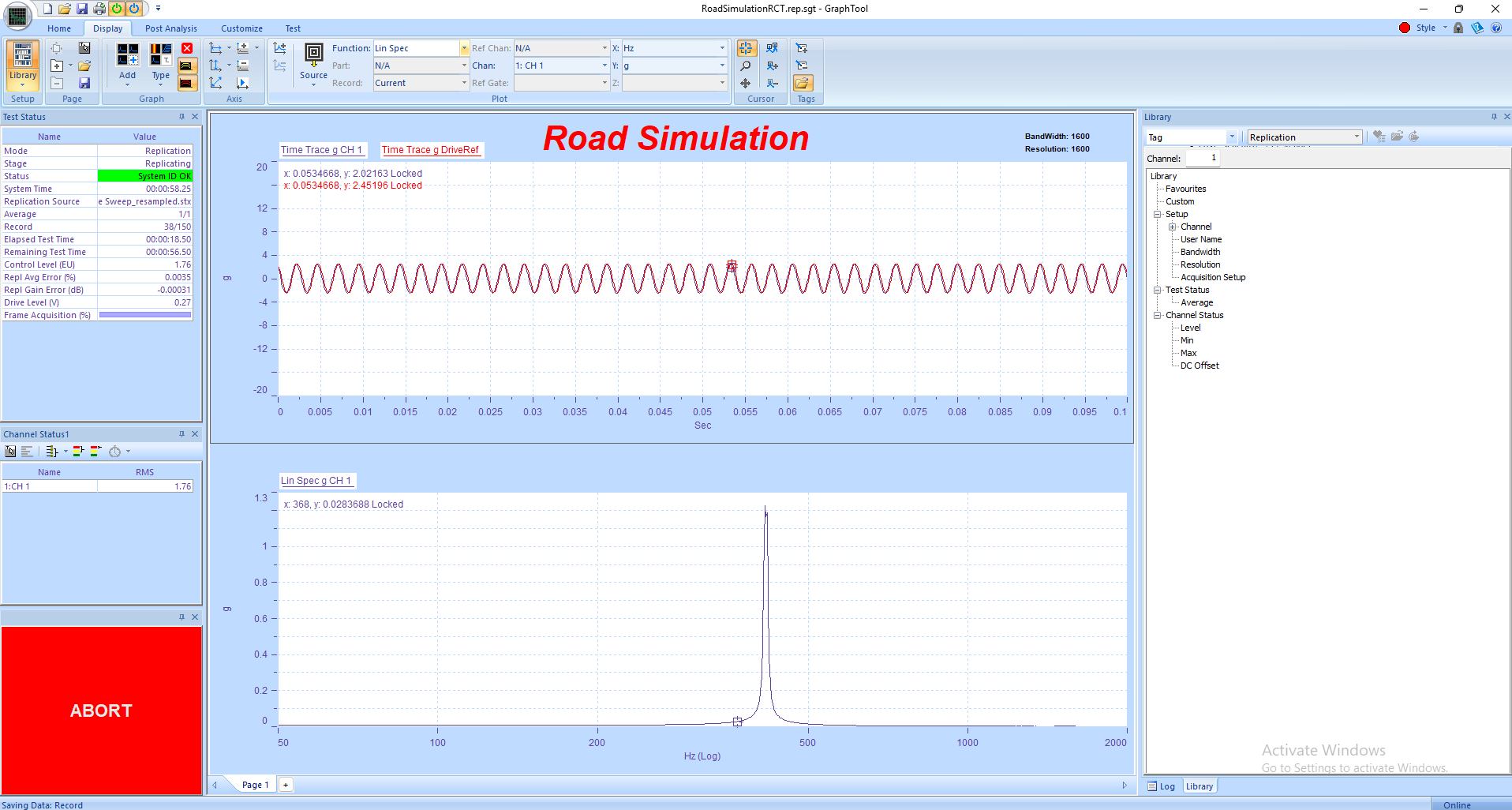
Utilizing the coherence function as an indicator of compensation quality is paramount to success. In addition, the coherence is also used as a tool in evaluating real time updates to the compensation function. The non shock applications have issues in that the desired reference waveforms are not statically defined as with the Shock reference pulse. For example, consider the replication of a swept sine wave in Road Simulation. In this case, the output waveform has a very narrowband signal, yet the compensation function is, by definition, a broadband function in nature. Any real time compensation update during replication would likely degrade the compensation function due to large spectral regions of the excitation function that were not properly excited at the same time. Degradation of the compensation function is what causes the undesired instability of the shaker output. 

Coherence is not always a good indicator in these applications because we’re dealing with single measurements, where the coherence is by definition equal to 1. Therefore, some additional parameters are needed to further restrict the real time update of the compensation function.

The Max Below (dB) compensation dialog field specifies a dynamic spectral level in the excitation spectrum (i.e. current reference waveform spectrum) to be used as a spectral line requirement for any compensation update. In our sine example, the current Sine reference spectrum would only have energy at or near the current drive frequency; all other spectral lines that lie below the threshold will not be used in any spectral update of the compensation function. By doing this, spectral lines that do not have a reasonable excitation level are omitted from the update process. As mentioned earlier, this field is not related to Shock compensation updates.

Updates to the SYSID Function (Shock)
Once a properly equalized compensation function has been established, further refinements can be incorporated with each successive output event. This process allows the compensation to be tuned for final output level conditions. Once established, the compensation can be Saved and Recalled. In addition, with each change performed on the compensation function, the prior compensation is automatically archived. This archival process allows the user to “unwind” any change that may have adversely affected the overall error in reference pulse output. Changes to the existing compensation are limited by several feedback parameters as defined in the System ID dialog under the Compensation group of parameters. When an output occurs, an internal error function is generated based on the ideal reference versus the measured response. Error corrections (aka feedback) will be made by using the designated Feedback Factor in correction magnitude. Because the corrections are based on individual measurements, one generally limits the correction factors to avoid large swings in amplitude changes. Note that all changes are performed on the frequency domain compensation function.

Remember that in most cases, the initial system ID is usually the best descriptor of the system response. Not all shaker/output systems respond in a truly linear fashion. Parametric effects on linearity often include amplitude level changes, external load factors, frequency content and test range as well as temperature variations. Sometimes, as one increases the output dB test level, the reproduction accuracy may degrade. Usually the issue is most apparent in the peak amplitude. One should resist the tendency to just constantly update the Hf function. Such updates will possibly modify the entire spectral content. If the basic shape of the output waveform is still good, we would recommend using the NLAF factor to adjust amplitude to get the peak correct and not muddy the original system ID with lots of updates trying to just tune in the amplitude. This method has proven very effective with nonlinear gain response found in various long stroke shaker systems.

In Shock, once a valid compensation has been generated, the user can optionally reuse that compensation function for additional tests, provided that the test setup parameters have not been altered. This feature is invoked with the ReStart of the test operations. Again, one should be cautious to ensure the shaker gain characteristics have not been altered between tests.

Updates to the SYSID Function (Non Shock Applications)
Non Shock applications include Waveform Replication, Sine on Random and Random and Random. These applications depend on a continuously generated output waveform while using the SYSID generated frequency response function to define an output shaping filter to compensate the reference waveform for output system’s characteristics. Because of the continuous nature of the output, SYSID updates are handled differently. For these applications, the system will build up an average error function which will be used to dynamically modify the System ID function while the test is running. In order to perform the necessary calculations, the error function will be built from a running average count as specified in the parameters.